Machine learning correlations of vectors
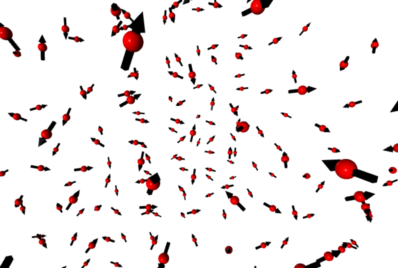
How could one identify the correlation patterns of the vectors uniformly distributed on a grid as shown in the image below? Instead of checking by eyes or matching different patterns speculated, unsupervised machine learning was applied which appears to be simpler, more efficient and more reliable.
Loading and visualizing the data
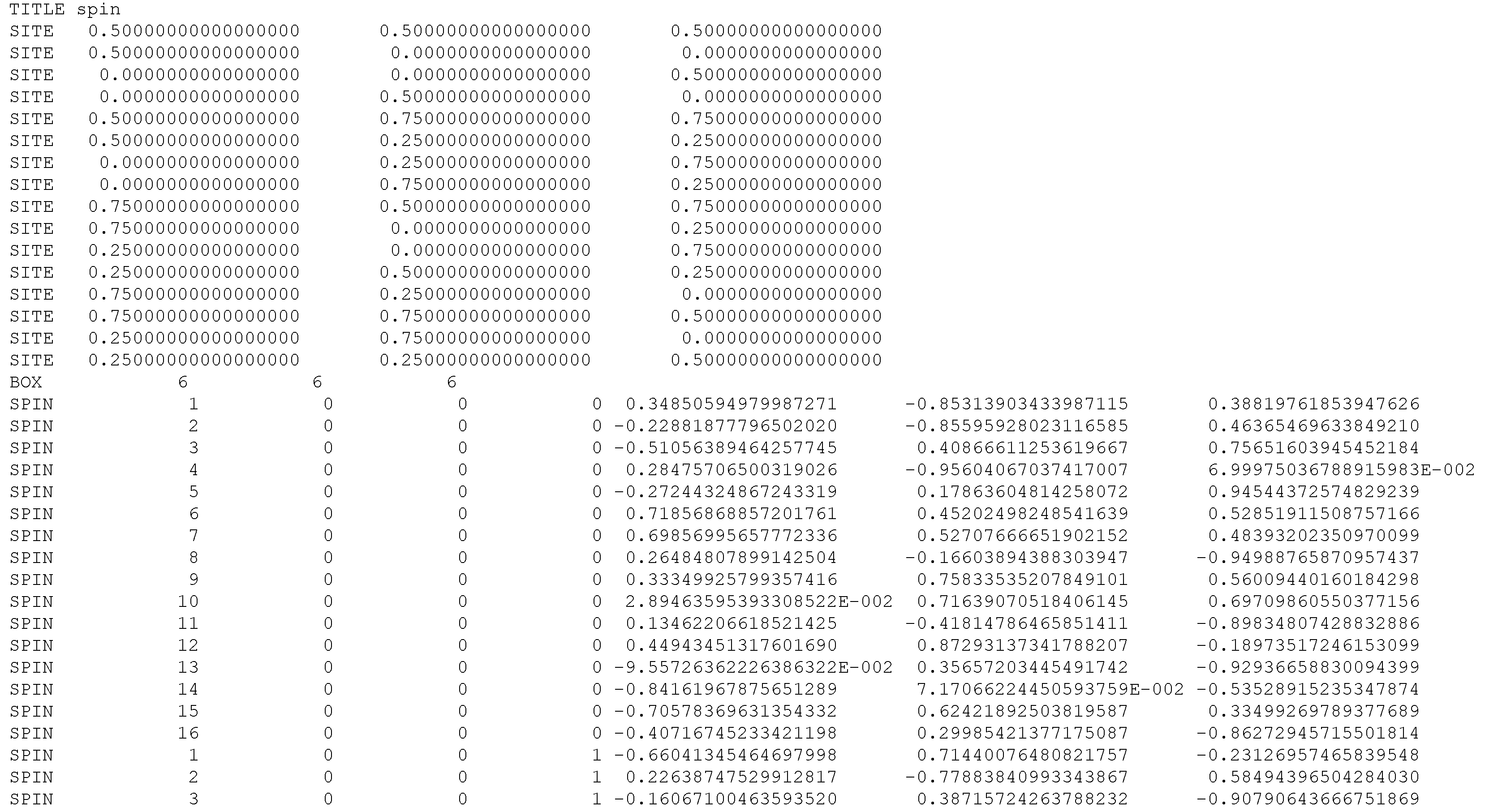
There are 50 independent datasets and each dataset contains 3456 vectors. Because the grid is uniform, the position information is simplified to the smallest repeated unit cell and the unit cell index \(x,y,z\). The unit cell contains 16 vectors at different positions and there are \(6\times6\times6\) unit cells per dataset. The postions in a unit cell in given in the header of the data file. The data are given in the following section with each row being \(x,y,z,i,S_x,S_y,S_z\), where \(i\) is the index in the unit cell and \(S_x,S_y,S_z\) are the three vector components.
Therefore, it convenient to store the data in a multi-dimensional array of Numpy. The shape of arrays storing the vector positions and vector directions are [50, 6, 6, 6, 16, 3]. The vector configuration can be visualized using the VPython (see the figure above).
Python code
import os
import fnmatch
import matplotlib.pyplot as plt
import matplotlib as mpl
from vpython import*
import numpy as np

# Loading all data
filepath = 'D:/Data/'
filename = 'spins*.txt'
ii=0
for file in os.listdir(filepath):
    if fnmatch.fnmatch(file, filename):
        if ii==0: #get the atom positions for the 1st file
            with open(os.path.join(filepath,file), 'rU') as f:
                i=0
                for line in f:
                    line=line.rstrip('\n').split()
                    if line[0]=="SITE":
                        atpos[i,:]=line[1:]
                        i=i+1
            with open(os.path.join(filepath,file), 'rU') as f:
                for line in f:
                    line=line.rstrip('\n').split()
                    if line[0]=="SPIN":
                        idxsp=np.array(line[1:5],dtype='int32')
                        poss[ii,idxsp[1],idxsp[2],idxsp[3],idxsp[0]-1,:]=idxsp[1:4]+atpos[idxsp[0]-1,:]
                        spins[ii,idxsp[1],idxsp[2],idxsp[3],idxsp[0]-1,:]=line[5:8]
            ii=ii+1
        else:
            with open(os.path.join(filepath,file), 'rU') as f:
                for line in f:
                    line=line.rstrip('\n').split()
                    if line[0]=="SPIN":
                        idxsp=np.array(line[1:5],dtype='int32')
                        poss[ii,idxsp[1],idxsp[2],idxsp[3],idxsp[0]-1,:]=idxsp[1:4]+atpos[idxsp[0]-1,:]
                        spins[ii,idxsp[1],idxsp[2],idxsp[3],idxsp[0]-1,:]=line[5:8]
            ii=ii+1

# Visualization using VPython
from vpython import*

def my_vector(a_list):
    return vector(a_list[0],a_list[1],a_list[2])

scene = canvas(title='MagStr', width=500, height=500,x=500,y=500,
                center=vector(0.5,0.5,0.5), background=color.white,exit=False)

L = 0.3 # spin vector length
R = 0.05 # atom ball radius

for i in range(6):
    for j in range(6):
        for k in range(6):
            positions_uc = np.squeeze(positions[0,i,j,k,:,:])
            spins_uc     = np.squeeze(spins[0,i,j,k,:,:])
            for w in range(16):
                pointer = arrow(pos=my_vector(positions_uc[i]-L*spins_uc[i]/2), axis=my_vector(L*spins_uc[i]),color=color.black) # plot the spin vectors
                pointer = sphere(pos=my_vector(positions_uc[i]), color=color.red, radius=R) # polot the atoms
Principal component analysis
Data preparation
PCA is a statistical technique commonly used when many of the variables (e.g., the vector components here) are highly correlated with each other and it is desirable to reduce the number of variables to an independent ones. The covariance matrix is diagonalized and eigenvalues and eigenvectors are obtained in PCA. The eigenvalues represent the contributions of the corresponding eigenvectors to the variance of the data. The eigenvectors are the independent variable set which are linear combinations of the original variables.
Because only short-range correlations existing in the system, it is reasonable to analyze at the level of small clusters, e.g. tetrahedra, unit cells. Therefore, the data was re-organized into matrix with every row presenting the vector components on a single cluster. The resulting array has the shape of [102400, 12].
Python code
# The cluster is a tetrahedron
def load_1file_to_tetra(file, sc, nbatom):
    """
    file: *_spins.txt file roduced by SPINVERT
    sc: one dimension of the super cell assuming the  supercell is (sc,sc,sc)
    nbatom: nb of spins per unit cell
    """
    temp = np.zeros([nbatom, 3])
    spins=np.zeros([sc*sc*sc*5, 4*3]) # 5 tedrahedra per unit cell, 4 spins per tetrhedron, 3 components per spin

    tetra = np.array([[0,4,8,13],
                      [1,5,9,12],
                      [2,6,10,15],
                      [3,7,11,14],
                      [0,5,11,15]])

    ii = 0
    idx = 0
    with open(file, 'r') as f:
        for line in f:
            line = line.rstrip('\n').split()
            if line[0]=="SPIN":
                temp[idx,:] = line[5:8]
                idx += 1
                if np.remainder(idx, 16) == 0:
                    spins[ii:ii+5,:] = np.squeeze(temp[tetra,:].reshape(5,-1,12,order='F'))
                    idx = 0
                    ii += 5
    return spins

def load_all_to_tetra(file_folder, file_name_pattern, sc, nbatom):
    i = 0
    for file in os.listdir(file_folder):
        if fnmatch.fnmatch(file, file_name_pattern):
            temp = load_1file_to_tetra(os.path.join(file_folder,file), sc=sc, nbatom=nbatom)
            if i == 0:
                spins = temp
                i = 1
            else:
                spins = np.vstack([spins, temp])
    return spins

filepath=r'D:/Data/'
filename='spins_*.txt'
spins = load_all_to_tetra(filepath, filename, sc=6, nbatom=16)
Analysis
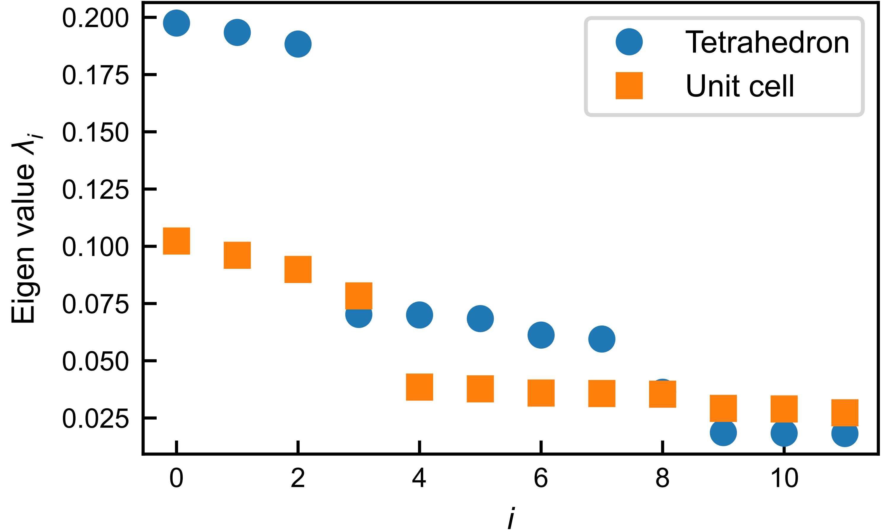
The matrix was fed to the standard PCA algorithm of the SciKit-Learn packages. The resulting eigenvalues are shown in the figure below sorted in descending order. Interestingly, there are three dominant principal components with nearly equal contributions ~20% to the variance, indicating three types of dominant degenerant correlation modes.
Additionally, the analyses at the level of the unit cell reveals a similar result except that the three dominant principle components explain less variance (\(\sim10\%\)) due to the short-range nature of the correlations and the averaging effect.
Python code
# PCA analyses on clusters
X = spins
print(X.shape)
n_components = 12
pca = PCA(n_components=n_components)
pca.fit(X)

X_reduced = pca.transform(X)
comps = pca.components_
print(pca.mean_)
Projection
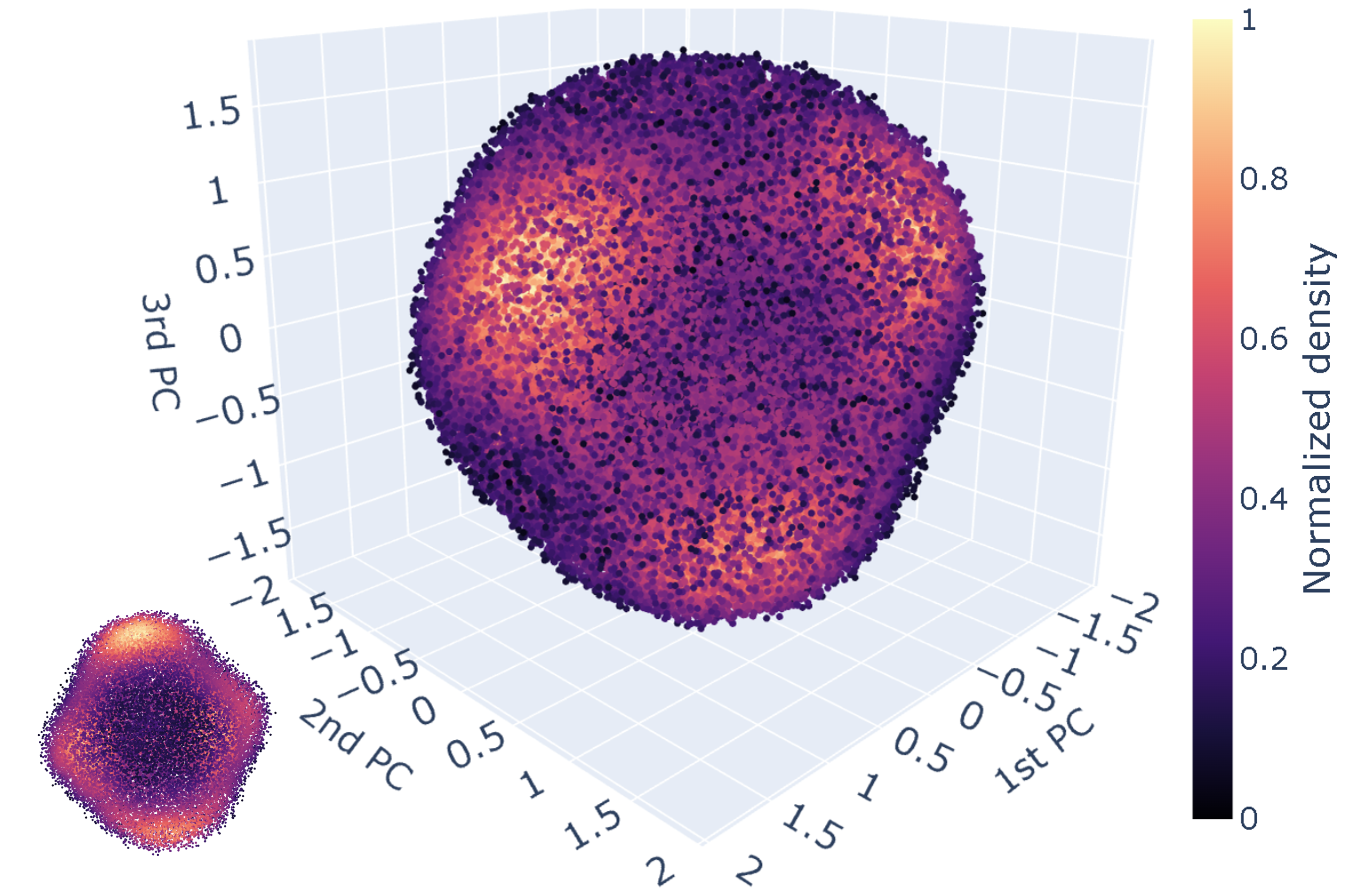
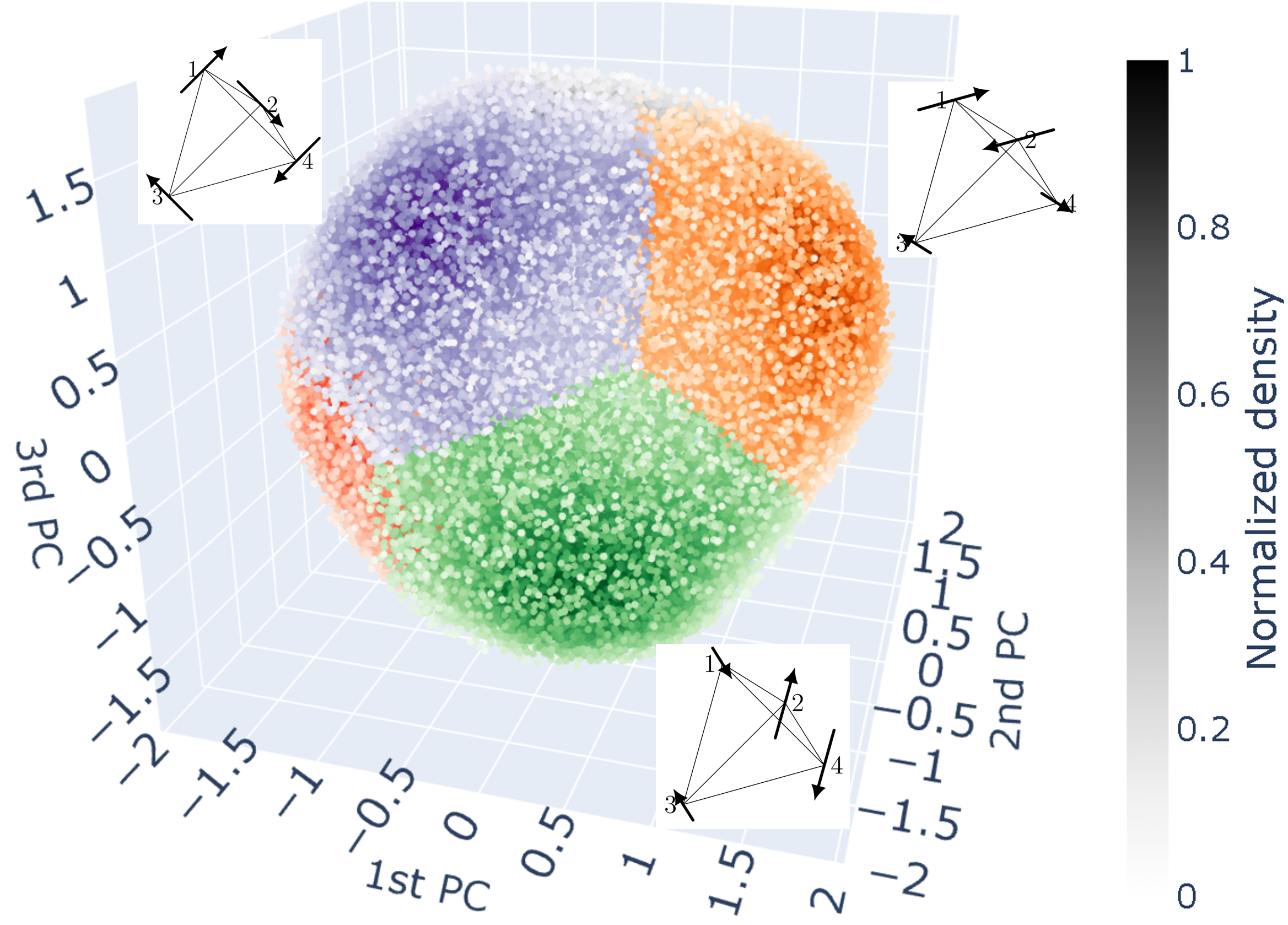
The vector configurations of the clusters can be conveniently projected into the three-dimensional space formed by the first three principal components (figure below). In the figure, each point represents a vector configuration on a single tetrahedron and the color indicates the density of points in respective regions. We can see that the points are mostly distributed on a spherical surface as a result of the fixed length of vectors and there are six high-density regions. Three are visible in the current view and the other three are on the back side of the sphere.
Python code
from scipy import stats
import plotly.graph_objects as go

xyz = X_reduced[:, 0:3].T
x, y, z = np.vsplit(xyz,3)
kde = stats.gaussian_kde(xyz)
density = kde(xyz).reshape([1,-1])

fig = go.Figure(data=[go.Scatter3d(x=np.squeeze(x), y=np.squeeze(y), z=np.squeeze(z),
                                   mode='markers',
                                   marker=dict(size=2,
                                               color=np.squeeze((density-density.min()) / density.ptp()), # set color to an array/list of desired values
                                               colorscale='magma',   # choose a colorscale
                                               colorbar=dict(title='Normalized density',titleside='right',
                                                             x=0.9,y=0.4,
                                                             len=0.7, thickness=20))
                                  )
                     ]
               )

fig.update_layout(
    autosize=False,
    width=800,
    height=800,
    scene = dict(xaxis_title='1st PC',
                 yaxis_title='2nd PC',
                 zaxis_title='3rd PC'),
    margin=dict(
        l=50,
        r=50,
        b=100,
        t=100,
        pad=10),
    paper_bgcolor="White",
    font=dict(size=15)
)
fig.show()
K-Means clustering
The centers of the high-density regions were of interests because they stands for the preferered vector configuration of the system. The centers can be obtain by clustering in the reduced space formed by the first three PCs using the standard unsupervised machine learning algorithm, K-Means.
Analysis
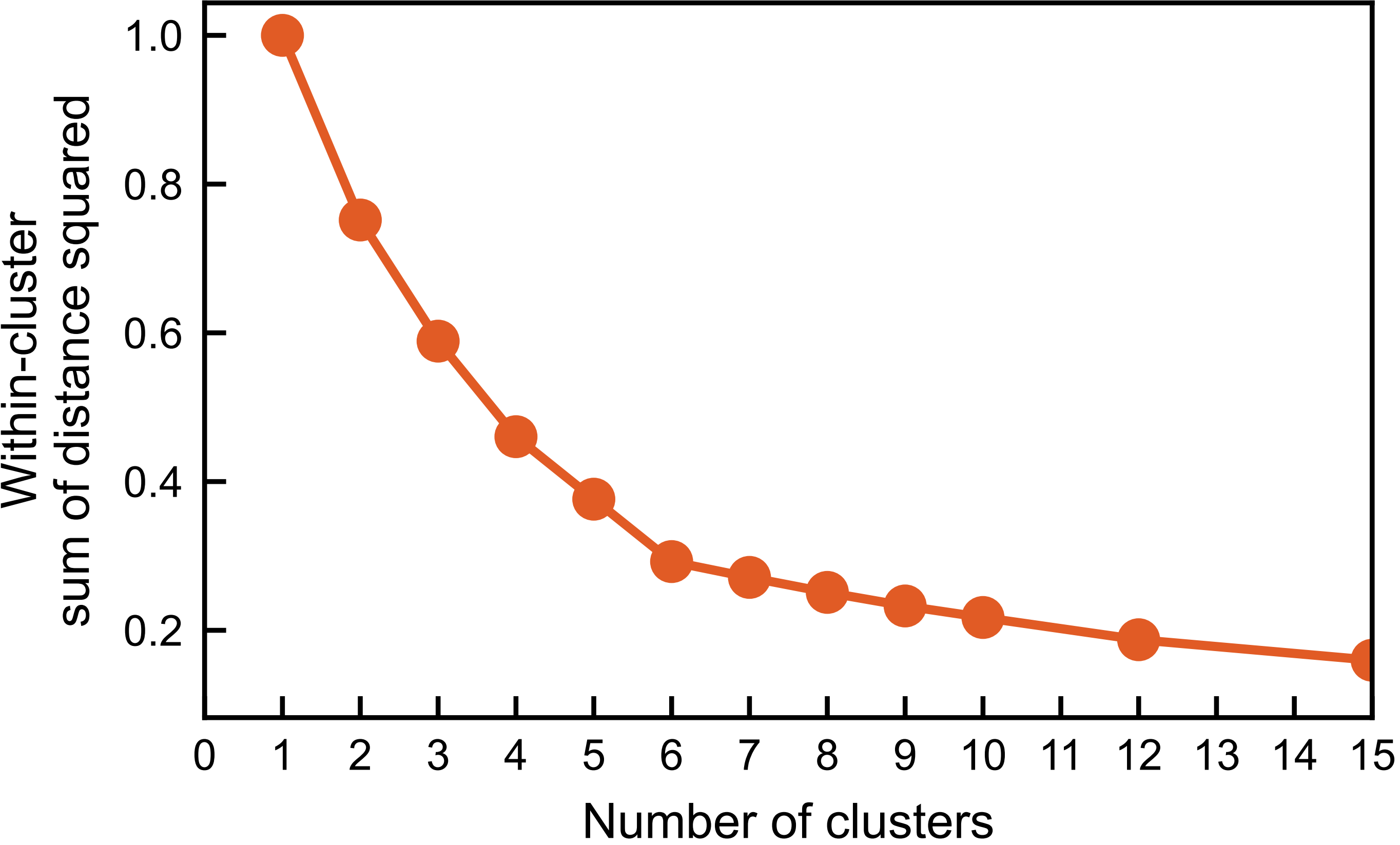
K-Means analyses with different number of clusters results in a elbow-shaped curve for the within-cluster sum of the squared distance. The six clusters were indeed identified and their coordinates can be obtained accordingly. The corresponding vector configurations on the tetrahedra in the original xyz coordinate system can be calculated by linear combinations of the three principal components with the coordinates of the centers as the corresponding coefficients. The vector configuration is found to the Palmer-Chalker type predicted for the pyrochlore antiferromagnet with dipole-dipole interactions.
Python code
from sklearn.cluster import KMeans

# Test with assuming different number of clusters
xyz = X_reduced[:, 0:3].T
x, y, z = np.vsplit(xyz,3)

n_clusters = np.array([1,2,3,4,5,6,7,8,9,10,12,15,20])

inertias = np.zeros_like(n_clusters)
for idx, i in enumerate(n_clusters):
    estimator = KMeans(n_clusters=i, n_init='auto')
    estimator.fit(xyz.T)
    inertias[idx] = estimator.inertia_

plt.figure()
plt.plot(n_clusters, inertias/np.max(inertias),'o-',c='#E25C25')
plt.gca().xaxis.set_major_locator(plt.MultipleLocator(1))
plt.xlabel('Number of clusters')
plt.ylabel('Within-cluster\nsum of distance squared')
plt.xlim([0,15])
plt.show()

# Assuming 6 clusters
estimator = KMeans(n_clusters=6)
xyz = X_reduced[:, 0:3].T
x, y, z = np.vsplit(xyz,3)
estimator.fit(xyz.T)
labels = estimator.labels_

# Re-presenting at the cluster centers in the original xyz coordinate system
spins_at_centers = (estimator.cluster_centers_@comps[0:3,:] + pca.mean_).reshape(6,3,-1) #in the original space
print(np.round(spins_at_centers,decimals=2))

normed = spins_at_centers/np.broadcast_to(
    np.absolute(spins_at_centers).max(axis=1).reshape(6,1,-1),(6,3,4))# 16 for uc, 4 for tetra

print(repr(np.round(normed).astype(int)))
Plot the clusters
The three clusters and the corresponding vector configurations in the real space are shown in the following figure. There remaining three clusters on the back side represent the vector configurations with reversed directions of the three visible one.
Python code
fig = go.Figure()
colors = ['Greys','Greens','Purples','Reds','Oranges','Blues','Blues']
density = np.squeeze(density)

for i in range(6):
    mask = labels.astype(float).reshape(1,-1) == i

    if i==0:
        print(np.sum(mask))
        fig.add_trace(go.Scatter3d(x=np.squeeze(x)[mask], y=np.squeeze(y)[mask], z=np.squeeze(z)[mask],mode='markers',
                                marker=dict(size=2,
                                                color=np.squeeze( (density[mask]-density[mask].min()) / density[mask].ptp() ), # set color to an array/list of desired values
                                                colorscale=colors[i],  # choose a colorscale
                                                #colorbar=dict(title='Normalized density',titleside='right',x=0.9,y=0.4,len=0.7, thickness=20)
                                                )
                                    )
                    )
    if i in [1,2,3,5]: # cluster 4 is masked out, giving zero lenght for color scale and error
        print(np.sum(mask))
        fig.add_trace(go.Scatter3d(x=np.squeeze(x)[mask], y=np.squeeze(y)[mask], z=np.squeeze(z)[mask],mode='markers',
                                marker=dict(size=2,
                                            color=np.squeeze( (density[mask]-density[mask].min()) / density[mask].ptp() ), # set color to an array/list of desired values
                                            colorscale=colors[i]  # choose a colorscale
                                            )
                                )
                    )

fig.update_layout(
    autosize=False,
    width=800,
    height=800,
    margin=dict(
        l=50,
        r=50,
        b=100,
        t=100,
        pad=10),
    paper_bgcolor="White",
    font=dict(size=16),
    scene = dict(
        xaxis = dict(visible=False),
        yaxis = dict(visible=False),
        zaxis =dict(visible=False)
        )
)

fig.show()
Conclusions
Hope now you know how manchine-learning is used in one of my research. It is more efficient and relable than the conventional method of defining an order parameter (a correlation mode).