Mean field calculation for spin models
Introduction
In physics and probability theory, Mean-field theory (MFT), analyzes the behavior of high-dimensional stochastic models by approximating them with a simpler model that averages over degrees of freedom. These models examine the interactions of numerous individual components.
The core concept of MFT is to replace the interactions affecting each individual component with an average or effective interaction. This transformation simplifies a complex many-body problem into a more manageable one-body problem. The simplified approach of MFT allows for gaining insights into the system’s behavior at a reduced computational cost. Here, I used the MFT to calcuation the dynamical correlation functions of a spin model on a pyrochlore lattice.
Theoretical background
The pyrochlore lattice
The pyrochlore lattice is described as a network of corner-sharing tetrahedra. Spins on the vertices of the lattice interact with each other. Physically, the nearest neighbor interactions are dominant and are commonly considered. The image below shows part of the infinite pyrochlore lattice, highlighting a few nearest neighbor interactions (\(J\)) for a spin.
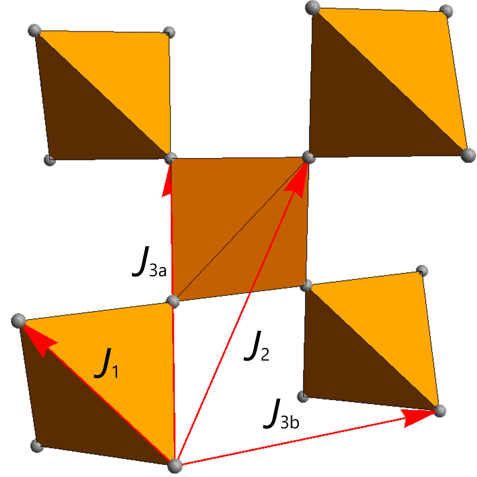
The pyrochlore lattice is a non-Bravais lattice containing 16 sites. To reduce redundancy and increase computational efficiency, we reduce the unit cell to the primitive rhombohedral unit cell with four sites.
The unit cell bases are \(a=(0,1/2.,1/2.), b=(1/2.,0,1/2.), c=(1/2.,1/2.,0)\).
The four sites are \(d_\nu = {(0,0,0), (1/4,1/4,0), (1/4,0,1/4), (0,1/4,1/4)}\).
The thoery
The spin Halmitonian can be written in the general quadratic form \begin{equation} H = - \sum_{n, \nu, \alpha, n’, \nu’, \beta} J_{n, \nu, \alpha; n’, \nu’, \beta} S_{n, \nu, \alpha} S_{n’, \nu’, \beta}, \end{equation} where \(S_{n,\nu,\alpha}\) is the \(\alpha\) component (\(\alpha=x,y,z\)) of the spin on the site \(d_\nu\) (\(\nu=1, 2, 3, 4\)) in the primitive unit cell located at \(t_n\). In the mean field theory, the magnetic structure is determined by the Fourier transformation of the Hamiltonian \begin{equation} J_{\mathbf{q}; \nu, \alpha; \nu’, \beta} = \sum_{n} J_{n, \nu, \alpha; n’, \nu’, \beta} \exp[i\mathbf{q}\cdot(t_n-t_{n’}+d_\nu-d_{\nu’})], \end{equation} where \(\mathbf{q}\) is a wavevector in the first Brillouin zone. The resulting \(J_{\mathbf{q}; \nu, \alpha; \nu', \beta}\) is a \(12\times 12\) Hermitian matrix which can be diagonalized: \begin{equation} \sum_{\nu’, \beta} J_{\mathbf{q}; \nu, \alpha; \nu’, \beta} u_{\mathbf{q}; \nu’, \beta}^{(\rho)} = \lambda_{\mathbf{q}}^{(\rho)} u_{\mathbf{q}; \nu, \alpha}^{(\rho)}\;, \end{equation} where \(\lambda_{\mathbf{q}}^{(\rho)}\) with \(\rho = 1, 2, ..., 12\) represents the eigenvalues and \(u_{\mathbf{q}}^{(\rho)}\) represents the corresponding eigenvectors. The global maximum of \(\lambda_{\mathbf{q}}^{(\rho)}\) determines the ordering transition with the transition temperature \(T_c\) as \begin{equation} k_{\rm B} T_{\rm c} = \frac{2}{3}[\lambda_{\mathbf{q}}^{(\rho)}]_\textrm{max}. \end{equation}
The paramagnetic susceptibility at a mean field temperature \(T_\textrm{MF} > T_c\) can be approximated by the eigenvalues and eigenfunctions: \begin{equation} \chi_{\mathbf{q}; \nu, \alpha; \nu’, \beta} = \frac{N \mu^{2}}{V} \sum_{\rho} \frac{ u_{\mathbf{q}; \nu, \alpha}^{(\rho)} u_{\mathbf{q}; \nu’, \beta}^{(\rho)*} } { 3 k_{\rm B} T_{\rm MF} - 2 \lambda_{\mathbf{q}}^{(\rho)} }, \end{equation} where \(N\) is the total number of the unit cell, \(V\) is the volume of the system, and \(\mu\) is the size of the magnetic moment.
The calcualtion can be directly compared to the experimental data. The cross section of the magnetic scattering can be expressed as
\[\begin{align} \frac{d \sigma}{d \Omega} & (\mathbf{Q} = \mathbf{G} + \mathbf{q}) = C f(Q)^{2} \sum_{\alpha, \beta, \nu, \nu'} \left( \delta_{\alpha \beta} - \hat{Q}_{\alpha} \hat{Q}_{\beta} \right) \notag \\ &\times \chi_{q; \nu, \alpha; \nu', \beta} \exp \left[ \mathbf{G} \cdot \left( d_{\nu} - d_{\nu'} \right) \right], \end{align}\]where \(C\) is a constant, \(f(Q)\) the magnetic form factor and \(\mathbf{G}\) the reciprocal lattice vector.
Numerical calculation
Find the nearest neibours
We include the interactions truncated at the third nearest neighbor. All such nearest neighbors for the four sites in a primitive unit are identified. We define a function for searching neighbors in a large supercell. The interaction properties (the bond length, site type, and displacement) are stored in a matrix. For a site, there are 6 nearest neighbors, 12 second nearest neighbors, and 12 third nearest neighbors of two different types.
Fourier transformation of the interactions
The Fourier transformation of the spin Hamiltonian is prepared as a matrix, with each element representing the sum of the interactions between two types of sites with the corresponding phase factor \(\exp(-i\mathbf{Q}\cdot \Delta r)\). We included magnetic dipolar interactions and exchange interactions.
Solve the Eigenproblem and Perform Calculations
The interaction matrix is symmetric and can be conveniently diagonalized. The eigenvalues and eigenvectors are used for calculations of the structure factor.
Python code
import numpy as np
from numpy import linalg as LA
from scipy import stats
from scipy import integrate
from scipy.optimize import minimize
from itertools import product, combinations_with_replacement

import os
import matplotlib.pyplot as plt

from numba import float64,jit,prange,njit, vectorize, guvectorize
from joblib import Parallel, delayed
import multiprocessing
multiprocessing.cpu_count()

# Atom positions in the premitive unit cell
r0=np.array([0, 0, 0])/4
r1=np.array([1, 1, 0])/4
r2=np.array([1, 0, 1])/4
r3=np.array([0, 1, 1])/4
rs=np.vstack([r0,r1,r2,r3]).T

# Unit cell bases
fcc = np.array([[0,1/2.,1/2.], [1/2.,0,1/2.], [1/2.,1/2.,0]])

# Supercell
scIdx = np.array(list(product([0,1,-1],repeat=3)))
sc = np.array([x[0]*fcc[0]+x[1]*fcc[1]+x[2]*fcc[2] for x in scIdx])

rss = np.array([rs[:,i]+sc[j] for i in range(rs.shape[1]) for j in range(len(sc))])
atomType = np.array([i for i in range(rs.shape[1]) for j in range(len(sc))], dtype=int)

def nn3(idAtom):
    """
	Function to find the 1st-3rd nearest neibours.
	idAtom: site index, a integer (0,1,2,3)
	Output: a 2D array
	"""
    dist = np.array([LA.norm(r-rs[:,idAtom]) for r in rss])
    idAtom2 = np.argsort(dist)[1:31]
    rAtom2 = rss[idAtom2]

    rij   = rAtom2 - rs[:,idAtom]
    typeAtom2 = atomType[idAtom2]

    bondCenters = np.array([r+rs[:,idAtom] for r in rAtom2[-12:]])/2.
    bondType = np.array([0,0,0,0,0,0,1,1,1,1,1,1,1,1,1,1,1,1])
    bondType = np.hstack([bondType , [2 if np.any(np.equal(rss,center).all(1)) else 3 for center in bondCenters]])
    return rij, typeAtom2, bondType, dist[idAtom2]

## Magnetic dipolar interactions
def DipMat(rij):
    """
	Magnetic dipolar interactions
	"""
    return np.array([1-3*rij[a]*rij[b]/np.sum(rij**2) if a==b else -3*rij[a]*rij[b]/np.sum(rij**2)
              for a in [0,1,2] for b in [0,1,2]]).reshape([3,3])

## Prepare the Matrix for Jex and Dip
rij, typeAtom2, bondType, DipMats = np.zeros([4,30,3]), np.zeros([4,30], dtype=int), np.zeros([4,30],dtype=int), np.zeros([4,30,3,3])
for i in [0,1,2,3]:
    rij[i,:], typeAtom2[i,:], bondType[i,:], _ = nn3(i)
    for j in range(30):
        DipMats[i,j,:,:] = DipMat(rij[i,j,:])

JexMats = np.zeros([4,4,3,3])

@jit(float64(float64[::1], float64, float64, float64, float64, float64, float64), fastmath=True, nopython=True, cache=True, parallel=False)
def Sq_3nnJexDip_fast(Q, Jex0, Jex1, Jex2a, Jex2b, Dip0, T):

    Dip1, Dip2 = Dip0/5.196, Dip0/8. #1.732**3, 2**3
    Jexs = np.array([Jex0, Jex1, Jex2a, Jex2b])
    Dips = np.array([Dip0, Dip1, Dip2, Dip2])

    HamJexDip = np.zeros((4,4,3,3))
    iMat =  np.identity(3)
    for i in range(4):
        for j in range(30):
            k, l = typeAtom2[i,j], bondType[i,j]
            HamJexDip[i,k,:,:] = HamJexDip[i,k,:,:] + (Jexs[l]*iMat - Dips[l]*DipMats[i,j,:,:])* np.cos(Q@rij[i,j,:])

    HamJexDip = np.transpose(HamJexDip, (0,2,1,3)).copy().reshape((12,12)).copy()
    val, vec = LA.eigh(HamJexDip) # eigh: orthorgnal vec for symmetric matirx; eig does not.

    Fq = np.transpose(np.sum(np.transpose(vec).reshape((12,4,3)), axis=1))
    Fq_perp = Fq - Q.reshape((3,1))@(Q@Fq).reshape((1,12))/np.sum(Q**2)

    return np.sum( np.sum(Fq_perp**2, axis=0) / (3*T*kb - val) )
Example
As an example, we calculate the structure factor in a reciprocal plane. Parallel computation can be performed for the loop to speed up the process. The pattern shown in the image below is characteristic for classical spin liquids.
Python code
x = np.linspace(-3, 3, num=121, endpoint=True)-3/121.
y = np.linspace(-4, 4, num=161, endpoint=True)-4/161.
X, Y = np.meshgrid(x, y)

# sqs = np.reshape([Sq_3nnJexDip_fast(2*np.pi*np.array([i,i,j]), 0.18, 0, 0,0, 0, 3.4) for i in x for j in y], (121, 161))
sqs = np.array(Parallel(n_jobs=8)(delayed(Sq_3nnJexDip_fast)(2*np.pi*np.array([i,i,j]), 0.18, 0, 0,0, 0, 3.4) for i in x for j in y))

plt.figure()
plt.pcolor(X, Y , sqs.T, cmap='jet')
plt.xlabel('X',labelpad=1)
plt.ylabel('Y',labelpad=1)
plt.colorbar()
plt.show()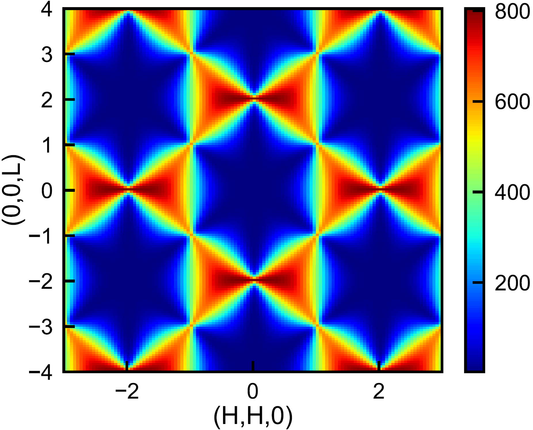
Summary
This article discusses using Mean-field theory (MFT) to analyze spin models on a pyrochlore lattice, a complex structure of corner-sharing tetrahedra. MFT simplifies the study of these systems by averaging interactions, reducing complexity and providing valuable insights into physical systems and experimental data before undertaking more complicated quantum calculations. I hope this gives you an understanding of how to perform MFT calculations.
