Monte Carlo and molecular dynamics simulations
Monte Carlo method is widely used to solve physical and mathematical problems. I have used this method to study a quantum spin ice system (see this paper Phys. Rev. Lett. 124, 097203(2020)). Here is a simple case: applying this method to a spin chain system. We first use this method with simulated annealing to find the ground state (global optimum) at low temperatures. Then we numerically integrated equation of motion (using Runge–Kutta fourth order method) with the ground state as the starting point to extract the temporal evolution of the state. At last, we can get the normal modes (energy-momentum relations of quasi-particle magnon excitations) of the system by doing a spacial-temporal Fourier transformation of the series states at different times.
Monte Carlo simulation
Implement the Monte Carlo algorithm
Here we define the function for Monte Caro simulations of a spin chain with only isotropic nearest-neighbour interactions (aligning spins parallelly or anti-parallelly). We initialize the state by randomly generating pointing directions for spins in unit length. Then, new spin directions are proposed successively for all the spins and will be accepted or rejected based the criteria \[ \text{Random(0,1)} < \exp\left[-\frac{\delta E}{k_\text{B}T}\right], \] where \(\delta E\) is the energy change if accept the new spin direction, \(k_\text{B}\) is the Boltzmann constant and \(T\) is the system temperature. The energy change is calculated based on the mean field created by the nearest-neighbouring spins and external magnetic fields, \[ \delta E = (\bf{S}_i^\text{new}-\bf{S}_i^\text{old})\cdot \bf{F}_i, \] with \(\bf{F}_i = J(\bf{S}_{i-1}+\bf{S}_{i+1})-H_\text{external}.\)
For speed purpose, we can update all the spins which are not interacting with each other simultaneously instead of iterating over all spin one by one. Here we take advantage of the internal parallel computing for matrix manipulation. Compare the two Monte Carlo functions MC_t and MC_t_fast defined below!
Python code
import numpy as np
from numpy import random
import matplotlib.pyplot as plt
from matplotlib.pyplot import cm
from matplotlib import colors
import vpython as vp
import time
def MC_t(J, H, T, S=None, n=20, nMC=1000, debug=False):
    """
    J: exchange interaction between nearest neigbour spins
    H: magnetic field: 1 by 3
    T: temperature in unit of J
    S: spin directions, num_of_spins by 3
    n: num_of_spins
    nMC:num of MC steps per spin
    """

    if S is None: # starting from a random spin configurations if not provided
        S = random.rand(n,3)-0.5
        S = S / np.sqrt(np.sum(S**2, 1))[:,np.newaxis]# normalize to unit length
    else:
        n = S.shape[0]

    acc = 0 # accumulating the num of acceptance
    for i in range(nMC):
        for k in range(n): # loop every spins and calculated mean field created by its two nearest neighbours
            if k==0:
                F = J* (S[n-1,:] + S[1,:]) - H # periodic boundary condition
            elif k==n-1:
                F = J* (S[n-2,:] + S[0,:]) - H # periodic boundary condition
            else:
                F = J* (S[k-1,:] + S[k+1,:]) - H

            # propose a new spin direction
            S_new = random.rand(3)-0.5
            S_new = S_new / np.sqrt(np.sum(S_new**2))

            # accept/reject: Metropolis condition
            dE = np.dot(S_new-S[k,:], F)
            if random.rand(1)[0] < np.exp(-dE/T):
                S[k,:] = S_new
                acc += 1
    if debug:
        print('Accept rate is: {:1.2f}'.format(acc/(nMC*n)), 'at T= {:1.5f}'.format(T))
    return S

def MC_t_fast(J, H, T, S=None, n=20, nMC=1000, debug=False):
    """
    Non-interacting spins are updated simultaneously, utilizing the advantage of internal parallel computing for matrix manipulation.
    Here the non-interacting spins are all the spins wiht even/odd index.

    Inputs:
    J: exchange interaction between nearest neigbor spins
    H: magnetic field: 1 by 3
    T: temperature relative to J
    S: num_of_spins by 3
    n: num_of_spins
    nMC:num of MC steps per spin
    Output: a spin configuration
    """

    if S is None:
        S = random.rand(n,3)-0.5
        S = S / np.sqrt(np.sum(S**2, 1))[:,np.newaxis]
    else:
        n = S.shape[0]

    acc = 0
    for i in range(nMC):
        # Preparing nearest neighbours
        S_rollU = np.roll(S,-1, axis=0) # next
        S_rollD = np.roll(S, 1, axis=0) # last

        # Update spins of even/odd index simutaniusly (parallel computing)
        for j in [0,1]:
            F = J * (S_rollU[j::2] + S_rollD[j::2]) - H[np.newaxis,:]
            n0 = len(F)
            S_new = random.rand(n0,3)-0.5
            S_new = S_new / np.sqrt(np.sum(S_new**2,axis=1))[:,np.newaxis]

            dE = np.sum((S_new-S[j::2])*F, axis=1)
            idx = random.rand(n0) < np.exp(-dE/T)

            S[j::2,:][idx] = S_new[idx]
            acc += np.sum(idx)

    if debug:
        print('Accept rate is: {:1.2f}'.format(acc/(nMC*n)), 'at T= {:1.5f}'.format(T))
    return S
Simulated annealing
Simulated annealing is a global optimization technique which is very useful for finding the ground state of the system. We annealing the system at high temperature and cooling down the temperature slowly. This is realised by doing a series of Monte Carlo simulations at lower and lower temperatures with taking the last high-temperature state as the starting point for the current lower temperature.
Python code
def anneal(J=1, H=np.array([0,0,0]), initT=1, endT=0.1, coolR=0.92, S=None, n=20, nMC=1000,debug=True):
    """
    Simulated annealing from hight temperature Ts[0] to Ts[-1]
    J: exchange interaction between nearest neigbor spins
    initT: staring high temperature in unit of J
	endT: the lowest temperature in unit of J
	coolR: cool rate (<1)
    S: num_of_spins by 3
    n: num_of_spins
    nMC:num of MC steps per spin for every temperature step
    """
    nSteps = np.int(np.log(endT/initT)/np.log(coolR) +1) # num of annealing steps

    # Estimate the time needed
    tic = time.time()
    S = MC_t_fast(J, H, initT, S=S, n=n, nMC=nMC,debug=False)
    toc = time.time()

    print(nSteps, 'anneal steps;', 'Time per step: {:1.0f} s;'.format(toc-tic), 'Total time needed: {:1.0f} s'.format((toc-tic)*nSteps))

    T = initT*coolR

    # annealing loop
    i = 1
    while T>endT:
        print('Anneal Step No. ', i)
        i += 1

        # Note: taking the state of the last T as the start for the current MC
        S = MC_t_fast(J, H, T, S=S, n=n, nMC=nMC, debug=debug)
        T = T * coolR

    return S, T
Results
Now we can run a anneal process to find the ground state of a ferromagnetic chains and visualize the spin configurations
Python code
n = 100 # nunber of spins on the chain
J = -1.0 # nearest-neighbour echange interactions
H = np.array([0,0.5,0]) # magnetic field
initT=0.5*np.abs(J)
endT=0.05*np.abs(J)
coolR = 0.9

S, T = anneal(J=J, initT=initT, endT=endT, coolR=coolR, S=None, n=n, nMC=1000)
S = MC_t_fast(J, H, endT, S=S, n=n, nMC=5000, debug=True) # more equillibrum steps at the lowest T
View the spin configurations using Vpython. Click on the figure to maximize it.
Python code
# Spin positions: chain along x direction
X = np.vstack([np.arange(n)-n/2, np.zeros(n), np.zeros(n)]).T
spinL = 1 # plot spin length
atomR = 1 # plot atom radius
cylR = 0.005 # plot bond thinckness

scene = vp.canvas(title='MagStr', width=1200, height=100,x=500,y=500, center=vp.vector(0,0,0), background=vp.color.black,exit=True)

for i in range(n):
    vp.arrow(pos=vp.vector(*(X[i]-spinL*S[i]/2)), axis=vp.vector(*(spinL*S[i]))) # spins
    vp.sphere(pos=vp.vector(*X[i]), color=vp.color.orange, radius=atomR*0.1) # atoms

for i in range(n-1):
    vp.cylinder(pos=vp.vector(*(X[i])), axis=vp.vector(*(X[i+1]-X[i])), radius=cylR, color=vp.color.gray(0.5))
Spin Dynamics from the equation of motion
Equation of motion
Having an equilibrium state after sufficient number of Monte Carlo steps at the base temperature, we can calculate the temporal evolution of the spin configurations. The spins process about the mean field created by the neighbouring spins and the deriv of the spin directions over time is given by the equation of motion, \[\frac{\text{d}\bf{S}_i}{\text{d}t}= \bf{S}_i\times\bf{F}_i. \] We integrate the Equation of motion numerically using the Runge–Kutta fourth order method to getting a series spin configurations at successive time stamps. Note the spin configuration at a time stamp is used for calculating that for the next time stamp. The time step size \(\delta t\) and number of time stamps \(Ndt\) are the parameters to tune. The \(\delta t\) controls the precision and \(\delta t \times Ndt\) is the length of the whole time span. The time span should be long enough to cover most of periods of the dynamical modes in order to capture most of the modes clearly.
Python code
# Derivative calculation
def deriv(J, H, S):
    """
    Deriv dS/dt calculation
    J: exchange interation constant
    H: 1 by 3 array for magnetic field
    S: num_of_spins by 3 for a spin configuration
    """
    n = S.shape[0]
    Fs = np.zeros_like(S)
    for k in range(n):
            if k==0:
                Fs[k] = J* (S[n-1,:] + S[1,:]) - H
            elif k==n-1:
                Fs[k] = J* (S[n-2,:] + S[0,:]) - H
            else:
                Fs[k] = J* (S[k-1,:] + S[k+1,:]) - H
    return np.cross(S, Fs)

def deriv_fast(J, H, S):
    """
    Deriv dS/dt calculation
    J: exchange interation constant
    H: 1 by 3 array for magnetic field
    S: num_of_spins by 3 for a spin configuration
    """
    n = S.shape[0]
    F = J*(np.roll(S,-1, axis=0) + np.roll(S, 1, axis=0)) -H[np.newaxis, :]
    return np.cross(S, F)

# Numerical integration
def Runge_Kutta(func, x0, Ndt=100, dt=0.01):
    """
    func: function to calculate the deriv
    x0: starting point
    Ndt: num of time stamps
    dt: time step size

    Return: y at different times and an array of time stamps
    """

    ts = np.zeros(Ndt)
    x = x0
    y = np.zeros(np.hstack([Ndt, x0.shape]))
    y[0] = x0

    print(y.shape)
    for i in range(1, Ndt):
        DD_1= func(x)*dt
        DD_2= func(x+DD_1/2)*dt
        DD_3= func(x+DD_2/2)*dt
        DD_4= func(x+DD_3)*dt

        # Spin configuration at t+dt
        ts[i] = ts[i-1] + dt
        x = x + 1/6*(DD_1 + 2*DD_2 + 2*DD_3 + DD_4)

        y[i] = x
    return y, ts

# Dynamics
def dynamics_FT1d(St, ts, xs, qs, omega):
    """
    Temporal and spacial Fourier transformation for a one-dimensional spin chain.
    Input:
    St: n_times by num_of_spins by 3 array for spin configurations (num_of_spins by 3) at differt times
    ts: 1d array for the n_times time stamps
    xs: 1d array for the n spin positions
    omega: 1d array for energies to calculated
    """

    qphase = np.exp(1j *2*np.pi*np.matmul(qs,xs)) # phase factor due to different locations
    ophase = np.exp(-1j*np.matmul(ts.reshape([-1,1]), omega)) # phase factor due to different time

    sxqw = np.matmul(np.matmul(qphase, St[:,:,0].T), ophase)
    syqw = np.matmul(np.matmul(qphase, St[:,:,1].T), ophase)
    szqw = np.matmul(np.matmul(qphase, St[:,:,2].T), ophase)

    return np.absolute(sxqw**2+syqw**2+szqw**2)
Results
After doing the calculation and visualization. We can see that the spins are precessing collectively and the traits forms cones which is very similar to a spinning top after being disturbed.
Python code
# Calculation of the temporal evolution
St, ts = Runge_Kutta(lambda S: deriv_fast(J, H, S), S, Ndt=5000, dt=0.1)

# Visualizing the spin directions at different times of five spins at the center of the chain
scene1 = vp.canvas(title='MagStr', width=1300, height=300,x=500,y=500, center=vp.vector(0,0,0), background=vp.color.white, exit=True)
scene1.camera.pos=vp.vector(*([0,0,2]))

mid = np.floor_divide(n,2)
which_spin = np.arange(mid-2, mid+2+1)

for idx, i in enumerate(which_spin):
    vp.sphere(pos=vp.vector(*X[i]), color=vp.color.orange, radius=atomR*0.1) # atoms
    if idx<len(which_spin)-1:
        pointer = vp.cylinder(pos=vp.vector(*X[i]), axis=vp.vector(*(X[i+1]-X[i])), radius=cylR, color=vp.color.black)

which_time = range(0,500,1)
color = [colors.to_rgba(c)
          for c in cm.get_cmap('Reds')(which_time /np.max(which_time ))]

# Plot spins at different times in a loop; the time stamp is encoded by the arrow color
for idx, i in  enumerate(which_time ):
    for j in which_spin:
        vp.arrow(pos=vp.vector(*(X[j]-0*spinL*St[i,j,:]/2)),
                 axis=vp.vector(*(0.5*spinL*St[i,j,:])),
                 color=vp.vector(*color[idx][:3]), round=True, shaftwidth=0.01*spinL, headwidth=0.02*spinL)
#scene1.capture('cones.png')

Dynamical structure factor
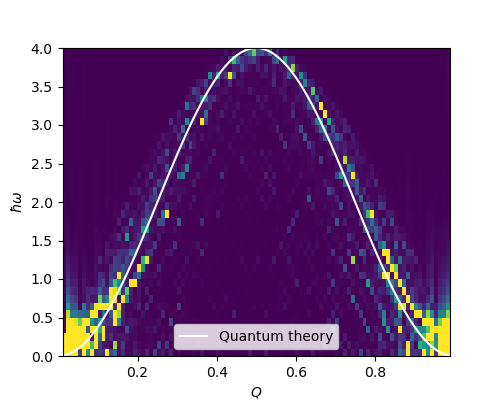
The movements of the spins propagate over the whole chain in the forms of normal modes which is wave-like (spin waves). We can use Fourier transformation to extract these normal mode from the spin configurations on the chain at successive time stamps. The energy-momentum relation of these normal modes (dispersion) for a ferromagnetic spin chains can be calculated using quantum mechanics (see the book Introduction to thermal neutron scattering by G. L. Squires), which is given by \[ \hbar\omega = 2J(\cos qa - 1), \] where \(\hbar\omega\) and \(q\) are the quasi-particle energy and momentum and \(a\) is the nearest-neighbour distance. We can see that the results of the simulated annealing and molecular dynamics is in good agreement with the quantum linear spinwave theory.
Python code
xs= np.arange(n).reshape([1,-1])
qs = np.linspace(1./n, 1, num=n-1, endpoint=False).reshape([-1,1])
omega = np.linspace(0, 5*np.abs(J), num=50, endpoint=False).reshape([1,-1])

def dynamics_FT1d(St, ts, xs, qs, omega):

    qphase = np.exp(1j *2*np.pi*np.matmul(qs,xs))
    ophase = np.exp(-1j*np.matmul(ts.reshape([-1,1]), omega))

    sxqw = np.matmul(np.matmul(qphase, St[:,:,0].T), ophase)
    syqw = np.matmul(np.matmul(qphase, St[:,:,1].T), ophase)
    szqw = np.matmul(np.matmul(qphase, St[:,:,2].T), ophase)

    return np.absolute(sxqw**2+syqw**2+szqw**2)

sqw = dynamics_FT1d(St, ts, xs, qs, omega)


plt.figure(figsize=(5,4))
Xax, Yax = np.meshgrid(qs, omega)
plt.pcolor(Xax, Yax, sqw.T,vmin=0.0,vmax=1000000)
plt.xlabel(r'$Q$')
plt.ylabel(r'$\hbar\omega$')
plt.ylim([0,4])

# Quantum linear spin wave theory
plt.gca().plot(qs, -2*J*(1 - np.cos(2*np.pi*qs)) + np.sqrt(np.sum(H**2)), c='w', label='Quantum theory')
plt.legend()
plt.show()
Summary
In this post, we briefly go through the study of a interacting spin chain system using Monte Carlo and molecular dynamics simulations. I hope you have gotten the general idea how to use it for your studies. In the paper mentioned in the introduction, we investigated a three dimensional system with anisotropic spin interactions.


